Workshop #4: Demand Forecasting
This workshop is intended for Master’s students interested in learning more about Supply Chain Optimization using Lokad’s dedicated programming language “Envision”. Envision is a domain-specific language (DSL) - created by Lokad - dedicated to the predictive optimization of supply chains. In this workshop, we will address the subject of demand forecasting. We will start by exploring the dataset, with the goal of identifying the critical parameters used in our model. We will then transition from a point forecast model to a probabilistic one, followed by a discussion on common use cases and limitations.
The workshop should take between 5 to 10 hours to complete, depending on your programming skills. It is not necessary to have completed the previous workshops in the series (#1 Supplier Analysis, #2 Sales Analysis and #3 Distribution Network Analysis). To help you, the full documentation for Envision is publicly available at Envision Reference - Lokad Technical Documentation..
Note: the relevant links to complete this tutorial have been inserted in the text below.

Table of contents
Introduction
Company overview
CM is a fictitious European company selling outdoor clothing with retail stores in three countries: Germany, France, and Italy. CM also has a strong online presence. The company offers customers the ability to purchase their products online, with home delivery available for added convenience. In addition to their website, CM sells their products through various online platforms, such as Amazon and other e-commerce marketplaces. This allows CM to reach a wider audience and connect with customers who prefer to shop online.
The company was founded by a group of friends who were passionate about the outdoors and wanted to make quality outdoor clothing and sporting equipment more accessible to everyone.
The first store opened in Germany and it was an instant success. The store was filled with high-quality outdoor clothing and equipment that was both stylish and functional. The founders of CM believe that people should be able to enjoy the outdoors without sacrificing style or comfort.
CM quickly expanded to other European countries, opening stores in France and Italy. Each store has a unique style and atmosphere that reflects the local culture and environment. The stores are more than just retail spaces; they are community hubs where outdoor enthusiasts can come together to share their passion for adventure.
Demand Forecast
CM is looking to organize their next set of purchase orders to effectively meet the demands of the peak season, while ensuring there are no inventory shortages and avoiding excessive overstock of their products.
Historically, the company has been somewhat simplistic in estimating future needs, relying on past sales data modified by a growth percentage set by their marketing team. However, this approach is outdated and needs an overhaul. The challenge here will be to provide forecasts that are independent of their budget and marketing strategy. These forecasts will serve as a core input for an optimization of their purchase decisions.
Note: this workshop’s scope is limited to demanding forecasting. The optimization logic will be covered in a subsequent workshop. Moreover, this workshop is not intended to be a forecasting techniques course - though some forecasting concepts will be mentioned.
To accomplish this objective, we will leverage a forecasting tool called Autodiff, which is part of Envision, the programming language developed by Lokad. This tool is grounded in the principles of Differentiable Programming. In a nutshell, Differentiable Programming (DP) is a paradigm that enables the computation of gradients or derivatives through computer programs. In the context of forecasting, Differentiable Programming proves valuable as it enables us to optimize and fine-tune forecasting models more effectively with the ability to compute gradients for updating model parameters and optimizing functions.
More details can be found in Differentiable Programming - Lokad Technical Documentation.
Objectives of the Workshop
The goal of this session is to be able to forecast demand for each CM reference. The results will later be used (in a subsequent workshop) as one of the inputs for the financial optimization of CM’s purchase decisions.
The session is structured in 3 linear steps:
-
Explore available data to understand how to structure a demand forecasting model.
-
Craft an initial forecasting model in the form of point forecast (classic time series forecast),
-
Transform the time series model into a probabilistic forecast model and explore its use cases and limitations.
Useful Definitions
-
Differentiable Programming: Differentiable Programming (DP) is a programming paradigm at the intersection of machine learning and numerical optimization. Language-wise, Envision treats DP as a first-class citizen, blending it with its relational algebra capabilities. From a supply chain perspective, DP is of prime interest for both performing diverse forecasting tasks and solving various numerical problems.
-
Autodiff: Abbreviation of “automatically differentiated” or “automatic differentiation”. This refers to a code block used in Envision to operate a stochastic gradient descent.
-
Reorder Leadtime (RLT): The Reorder Lead Time (RLT) is the time-frame between two successive purchase orders. For instance, if the reordering process requires monthly orders, then the RLT would be about 30 days. The Reorder Lead Time is consequently the period covered by each new purchase order (for instance, if someone goes to the grocery store once every week, then the food purchased should ideally cover needs for a seven-day time-frame). Mainstream supply chain books also call this a “reorder period”.
-
Supplier Leadtime (SLT): Supplier Lead Time (SLT) refers to the time it takes for a supplier to fulfill an order and deliver the purchased goods to the buyer.
-
Underfitting: Underfitting is a situation where a predictive model is unable to capture the full extent of the statistical patterns between the input and output variables. As a result, the model is not as accurate as it could be, as it does not leverage all the patterns that are available in the dataset. It is typically said that an underfitted model has excessive bias, and not enough variance.
-
Overfitting: Overfitting is a situation where a predictive model goes beyond the capture of the statistical relationship being input and output variables. E.g., the model captures statistical noise and mistakes them as pattern. Empirically, the model has low error on the data set but much greater error once presented with unseen/fresh/new data. It is said that an overfitting model has excessive variance and not enough bias. See also Overfitting: when accuracy measure goes wrong.
-
Products clustering: Products clustering in predictive models involves grouping similar references based on common characteristics or features. This technique helps to identify patterns, relationships, or trends within the data, thus contributing to more accurate predictions.
Dataset
The dataset provided for this workshop consists of 4 tables (see the data schema below). They are preloaded in the Envision playground (see lines of code #2 to #36).
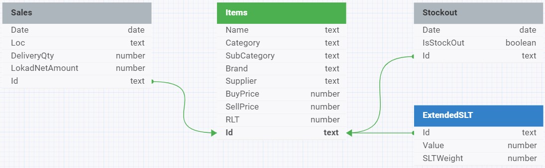
In this schema, green arrows indicate the relationships between the tables, specifically the foreign key to primary key relationships. These relationships are essential for joining tables in a relational database to query data across different entities.
For example, the Items table, which stores information about the company’s product catalog, is a central table with relationships to the Sales, Stockout, and ExtendedSLT tables through their foreign keys (as indicated by the green arrows). This implies that the .Id field in these tables references the primary key in the Items table, allowing for a relational link between the data in the different tables.
The arrow lines start from the foreign key side with the arrowheads pointing towards the primary key side, which is a typical way to denote the direction of the relationship from the foreign key in one table to the primary key in another.
1. Items Table (Catalog.tsv)
- Purpose: Details each item sold by CM.
- Contents: Includes item reference, product name, category, subcategory, brand, supplier, and both buying and selling prices.
- Key Fields:
Id(Item Reference),Name,Category,SubCategory,Brand,Supplier,BuyPrice(per 1 unit),SellPrice(per 1 unit).
2. Sales Table (Orders.tsv.gz)
- Purpose: Records all sales transactions to customers of CM.
- Contents: Includes item reference, date, location, quantity delivered, and net amount paid.
- Key Fields:
Id,Date(order date),Loc(location where the sale took place),DeliveryQty(the quantity in units delivered to the customer),LokadNetAmount(the amount in euro paid by the customer).
3. StockOuts Table (StockOuts.tsv)
- Purpose: Tracks instances of stock unavailability at CM.
- Contents: Records dates when specific items were out of stock.
- Key Fields:
Id,Date,IsStockOut.
4. ExtendedSLT Table (ExtendedSLT.tsv)
- Purpose: Provides lead time probability distributions in tabular form for each item.
- Contents: Includes item ids, their lead times, and respective lead time probabilities.
- Key Fields:
Id,Value(lead time in days for respective item),SLTWeight(decimal probability of respective lead time value for respective item).
Note: At present, our public Envision environment (try.lokad.com) doesn’t support ranvar datatype, which is a datatype for probabilistic forecasts. For this reason ranvar is replaced by its tabular counterpart consisting of Value and SLTWeight and respective workarounds in the code provided.
Part 1: Exploring the Dataset
Before starting to build our demand forecast, we must understand the business reality we are trying to model. Exploring the dataset will enable us to understand the orders of magnitude we are dealing with, and which parameters will be important to consider for our model.
Questions
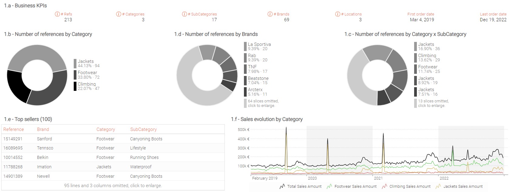
- Create a summary tile that display the following KPIs:
- Number of references
- Number of categories
- Number of Sub-categories
- Number of brands
- Number of locations
- First Order Date and Last order date.
This will help us to have a better understanding of the scope.
Hint: Use column
Locin Sales table.
-
Display the number of references by Category in a piechart tile.
-
Display the number of references by SubCategory in a
piecharttile. -
Display the number of references by Brand in a
piecharttile. -
Display in a table tile the following information for each reference belonging to the 100 top sellers over the last 365 days:
- reference identifier
- brand
- category
- subcategory
- reference name
- sales amount over 365 days
- sales rank amount.
-
Display in a linechart tile the Sales Net Amount for each Category by week.
-
Consider the following:
- Do all categories share the same sales profiles?
- Which parameters should be learned in our forecasting model, and at which level?
- Could other parameters be considered with additional data?
Conclusion
There are about 200 references in the scope divided into three categories and 17 subcategories. Each product category seems to have a different sales profile:
- Climbing products have a rather flat sales profile, without any significant trend or seasonality.
- Jackets do not seem to be on a growing trend but are subject to stronger sales at the end of the year and occasionally encounter substantial one-time spikes.
- Footwear demonstrates a robust sales increase, along with a high season at the end of the year.
From these observations, we will craft a forecasting model (detailed in the next part) for each reference that uses the following parameters in a weekly time frame:
- Level of sales (at Reference level)
For each reference, we want to know what the average weekly level of sales is. This is the basis for our forecast.
- Seasonality (at Category x Week level)
From the conclusions made above, products from different categories have different seasonality profiles. It is thus important not to mix them. For that, we will use different clusters of products using the product category attribute.
To avoid overfitting the rather short historical data, it is better to avoid calculating seasonality profiles at the reference level. Of course, other aggregation levels could have been suggested (such as the Subcategory level), and we could even use clustering methods to avoid being limited to aggregations directly available from the dataset. Seasonality computed on a weekly level seems to be the best choice here, as high seasons can stretch across different months.
- Trend (at Reference level)
As references from the same category are at different stages of their life cycles, it is preferable to learn the trend independently for each product. Other methods could be suggested, such as a decreasing sales profile depending on the number of weeks after product launch. In fact, this is a method that is often used for fashion products. That said, we opt here for a more straightforward approach.
Additional insights and data from the customer could lead us to consider additional parameters to improve our demand forecasting model. For example, if references are often subject to price variations (due to price increases on raw materials, discount periods, etc.), learning the demand elasticity to price variations would help us to better react to future changes.
Hint: To check yourself here is an example of a dashboard that you might build. The exact layout (and color) of the dashboard might be different depending on your choices.
Part 2: A Point Forecasting Model
Introduction
From Lokad’s experience, in supply chain management, costs are driven by extreme events: it’s the surprisingly high demand that generates stock-outs and customer frustration, and the surprisingly low demand that generates dead inventory and consequently costly inventory write-offs. When demand is exactly where it was expected to be, everything goes smoothly. As such, the core forecasting business challenge is not to do well on the easy cases (where everything will probably be fine using a crude moving average). The core challenge is to handle the tough cases; the ones that disrupt your supply chain, and drive everybody nuts.
This perspective led Lokad to advocate for a new way of tackling forecasts, namely probabilistic forecasts. Simply put, a probabilistic demand forecast does not merely give an estimate of demand; it does that and it assesses the probabilities of every single future demand scenario. E.g., the probability of 0 (zero) units of demand is estimated, the probability of 1 unit of demand is estimated, and so on. Every level of demand gets its estimated probability until the probabilities become so small that they can safely be ignored.
To dive progressively into forecasting, we will start by building a point concurrent time series forecast model. This first model will then be transformed into a probabilistic forecast. It is important to note that this part of the workshop strongly relies on the script provided and its associated dashboards.
Note: At Lokad, we favor low-dimensional parametric models, both for point forecasts and probabilistic forecasts. However, do not underestimate the capabilities of such models, as they do achieve state-of-the-art accuracy, even when pitted against hyperparametric models or non-parametric models.
Forecasting model
Following our observations from Part 1, we will be using the following parametric model:
$$Baseline_{[Items, Week]} = \exp( Level_{[Items]} ) \cdot Seasonality_{[Items, Week]} \cdot LinearTrend_{[Items, Week]}$$
The use of the the exponential function is a trick that will be explained in a dedicated question below.
The three parameters composing the $Baseline$ (which is our forecast) will be learnt by the autodiff block. This will be done by minimizing the “loss” through a series of iterations. The “loss” here is the mean square error (MSE):
$$\Delta^2_{[Items, Week]} = (Baseline_{[Items, Week]} - SmoothedDemand_{[Items, Week]})^2$$
This model is:
- Point: For every week and every product, the model returns only one value.
- Concurrent: The parameters are not intended to be trained in strict isolation from one product to the next. There is some implicit “coupling” between the series.
Questions
a. Manipulation of Raw Inputs
-
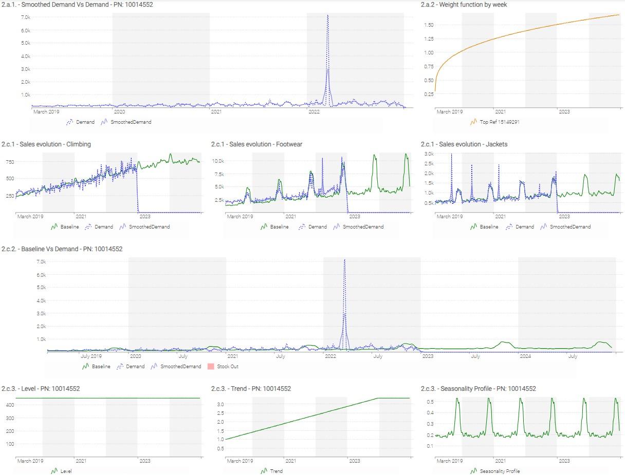
Looking at the linechart “2.a.1. - Smoothed Demand Vs Demand” for reference 11800905, explain why it is beneficial to use what we call a “smoothed sales history”? (Note: the formula used to compute a smoothed sales history is detailed in the code).
-
In the loss function we introduce $Weight$ depending on each week. This $Weight$ is expressed by the formula:
$$Weight_{[week]}=0.3 + 1.2 \cdot \frac{Weeknum_{[week]}}{TotalNumberOfWeeks}$$
Why is it beneficial to assign a different $Weight$ to each week for each reference?
Hint: the weekly evolution of the $Weight$ is displayed on the linechart “2.a.2 - Weight function by week” for the Top reference.
b. Initialization of Parameters (Subsidiary questions for people interested in gradient descent)
-
When it comes to learning parameters through a stochastic gradient descent, the question of parameter initialization is crucial. In our forecasting model, we could, for example, initialize the level for all items to 0. In your opinion, why is it beneficial to initialize the parameters learnt in our model with a quick approximation of the final value?
-
In your opinion, why are we using the
log()function when initializing the $Level$?
c. First Point Model
Hint: In this section we use the code lines written in “CODE BLOCK #1: FIRST AUTODIFF MODEL”.
-
For each category, display a
linechartrepresenting the sum of Raw Demand, Smoothed Demand & Baseline. How does each parameter impact the forecast for the different categories? From these aggregations, can we conclude that the forecast is of good quality? -
Display the same
linechart, but sliced by reference and including a representation of stock-out periods for the selected reference.
Hint: create slices using the syntax
table Slices[slice]= slice by Items.A title: Items.Awhere A is the vector representing the object used for slicing.
-
For each reference (use the slicing you created before), display in a
linecharttile the weekly level, trend and seasonality profile. -
Analyze the results for the 3 following references: 15149291, 12564089 & 11557472. What observations can be made? What could be changed in our first model to improve results?
Hint: Here is an example of a dashboard that you might build. The exact layout (and colors) of the dashboard might be different depending on your choices.
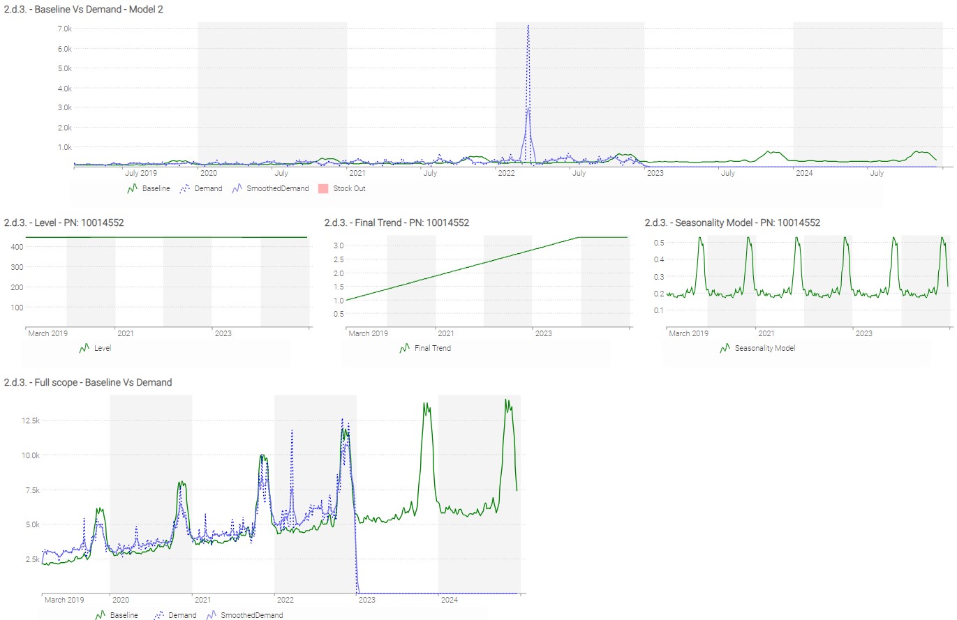
d. Second Point Model
Based on the above conclusion, poor management of stock outs diminishes the quality of the results (example ref 11557472). We also concluded that within a category there was some sub-clustering of products with different seasonality patterns. We’ll see in this second model how we can improve the management of both these details.
Hint: In this section we use the code lines written in “CODE BLOCK #2: SECOND AUTODIFF MODEL”.
- Management of Stock Outs
- Create for each reference a weekly coefficient that is equal to 1 when the given reference is in stock-out and to 0 when the reference is in stock.
- Adapt the “SECOND AUTODIFF MODEL” to consider the weekly coefficient defined above.
- Seasonality Management
- Which attributes could be used to better cluster items that share the same seasonality patterns?
- Assuming we’re using the subcategory instead of the category as seasonality clustering, adapt again the “SECOND AUTODIFF MODEL”.
- Display the same linecharts and check the new results for the same references listed previously in question 2.c.4). How did results evolve?
Conclusions
When building a forecasting model, an iterative approach will help obtain good results. To quickly identify the most useful improvements for your model, start the analysis from the final decisions using the forecast as input. For instance, in CM’s situation, reviewing odd purchase decisions can help identify issues in our forecasting model (of course, to do that you need to have a first version of a purchase optimization set up).
After analyzing the results for 3 different references, we decided to change the number of seasonality profiles per Category, filter out exceptional sales, and exclude stock-out periods from the sales history. Of course, reviewing purchase decisions for more examples could lead to additional changes.
Hint: Here is an example of a dashboard that you might build. The exact layout (and colors) of the dashboard might be different depending on your choices.
Part 3: A Probabilistic Forecasting Model
Regardless of the accuracy of the forecasting model, a point model will always present significant limitations. While it might provide a “best guess” of future demand, it says nothing about all the alternatives, and to which extent they are likely to occur.
This is a critical limitation of the point forecast, given that the extreme scenarios (e.g., exceptionally high or low demand) are precisely the ones that disrupt supply chains the most, and carry the most significant financial opportunities or penalties. As a result, decisions engineered on top of point forecasts are fragile by design. In order to make those decisions robust, probabilistic forecasts are needed.
At every point of time in the future, we can define a probabilistic demand instead of a single value.
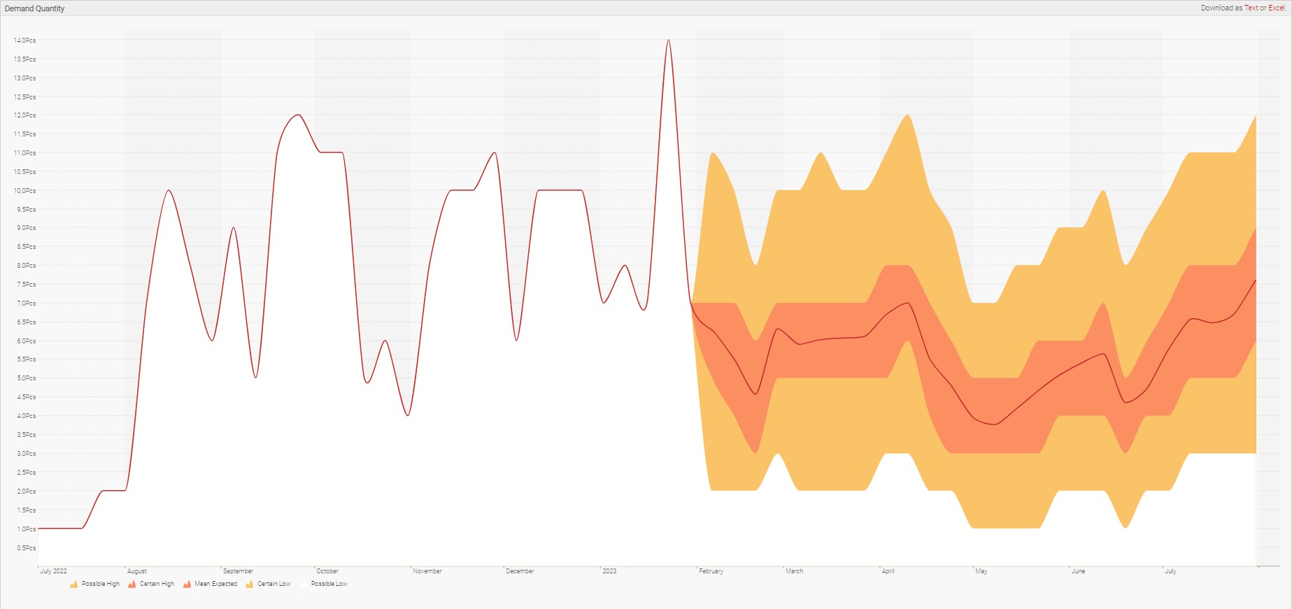
In the above diagram, future demand “starts” where the yellow-orange shotgun effect begins. This colored-effect represents the range of possible demand values, with the midpoint (most likely) value represented by the thinnest inner line.
Moving forward, we will use the term “probabilistic demand" or “distribution of demand” for the representation of all possible outcomes and their associated probability for a given time horizon.

As you can see in the above diagram, the most likely demand value is approximately 130, but surrounding demand values are similarly probable. If we sum up all the demand values, it will cover 100% of the likely demand scenarios.
There are two objectives for this third part of the workshop:
- First, we will understand the relevant temporal horizon regarding CM’s problem, bearing in mind that the associated business goal is to procure the right quantities for the upcoming high season.
- Second, we will compute a probabilistic demand for the chosen horizon.
Questions
a. Probabilistic Forecast
The relevant horizons
We will assume that usual sales volumes, supplier constraints (minimum purchase amounts), and available storage space force CM to place orders every month. We will use the acronym RLT (Reordering LeadTime) to refer to this purchasing frequency. This period will be expressed in days. As a reminder, the acronym SLT stands for Supplier Lead time (see useful definitions).
Assuming we place a new Purchase Order today (T), the quantities procured are intended to cover the time span between T + SLT and T + SLT + RLT.
To determine the required quantity, it is essential to consider various elements: demand variability, uncertainty of Supplier Lead Time, and total stock (Available and On Order).
In the coming questions, the intent is to cover the period from 1st of November 2023 to 31st of December.
-
Display the SLT distribution for the 3 top selling references (it is preferable to display
ranvarvalues inscalartiles). What can you conclude? -
When should you place your purchase order? Note: Assume that you want to make sure all products from supplier “TalonCotex” are delivered at the beginning of the period (the quantities purchased will cover the whole period).
Moving forward, we will consider that SLT is 50 days and RLT is 30 days for all references. Note: In real life it would be a mistake to avoid embracing uncertainty on leadtimes, but for the purposes of this exercise we will make this exception.
- For one reference, how many times will you place a Purchase Order to cover the period?
- For reference 15149291, display in a
linecharttile on a weekly basis: quantity sold and mean demand forecast. - On the same
linechart, display the high season period and the weeks where the 2 Purchase orders should be placed (hint: use “seriesType: background”).
Probabilistic demand calculated from the baseline
Now that we have identified the relevant temporal horizons, we will transform our point forecast into a probabilistic demand.
Many mathematical models used to calculate probabilistic demands are described in the academic literature. In this workshop, State Space Model is used. The probabilistic demand forecast over the RLT will be generated by successive draws from a negative binomial distribution. For each week composing the RLT (~4 weeks in total), the negative binomial parameters are:
- Baseline(t)
- Dispersion (independent of the week).
Lokad designed a function actionrwd.Segment() that generates the expected demand forecast. The function requires the following inputs:
TimeIndex: Defines a non-ambiguous ordering for each week composing the RLTBaseline: The baseline of the average demand for each weekDispersion: How erratic is the demand? The dispersion parameter (variance divided by mean) of the demandAlpha: to what extent are sales correlated from one week to another? For simplicity, we will consider that there is no correlation (alpha = 0),Start: The inclusive start of the segment expressed in periods (zero indexed)Duration: The length of the segment expressed in number of periodsSamples: number of trajectories
Hint: In this section we use the code lines written in the code section “N3: Probabilistic Demand”.
- Calculate the probabilistic demand over the first month of the coverage period. Compare the distribution with the sum of point forecast (baseline) from weeks between 30th of October and 27th of November (included).
- Which risks need to be considered when it comes to deciding what is the right quantity to purchase using a probabilistic forecast?
b. To go further
Time-wise dependencies
In the first probabilistic model, we have assumed that the sales quantities are independent from one week to another. This is a significant simplification as real life shows that this is wrong. A very good example is the sales volumes for a new book. If the sales in the initial days or weeks are strong, it likely indicates that positive word-of-mouth is increasing the book’s popularity, thus likely boosting sales for the following weeks. Therefore, incorporating the correlation between weekly sales is crucial for creating a coherent probabilistic forecast. The Innovation State Space Model (ISSM) considers this phenomenon. Thanks to the function actionrwd.Segment() already used above, we can compute a probabilistic forecast that factors time-wise dependencies.
Hint: In this section we use the code lines written in the code section “N4: Probabilistic Demand”.
- Calculate the probabilistic demand over the first month of the coverage period considering a 20% correlation between weeks.
- What can be said about the probabilistic forecast’s extreme scenarios?
Demand forecast accuracy
Introduction
Lokad’s take on this topic is quite different from what is typically taught.
Simply put, forecasting errors cost money to companies expressed in dollars, not in percentage. As such, the ideal metric should not measure value expressed as percentages of accuracy error. Rather, the metric should be expressed in Dollars or Euros, precisely reflecting the cost of the inefficiencies caused by the inaccurate forecasts.
While most popular metrics are symmetric (pinball loss being a notable exception), risks of overforecasting vs underforecasting are not symmetric in practice. Lokad suggests adopting a viewpoint where the metric is closer to an economic cost function – carefully modeled to fit the business constraints – rather than a raw statistical indicator.
Nevertheless, we are going to explore in this section some forecasting metrics that are sensitive when it comes to evaluating the accuracy of a probabilistic forecast.
Literature on forecast accuracy metrics encompasses various methods and approaches used to evaluate the performance of forecasting models. Commonly used forecast accuracy metrics include Mean Absolute Error (MAE), Mean Squared Error (MSE), Root Mean Squared Error (RMSE), Mean Absolute Percentage Error (MAPE), and Forecast Bias.
All those indicators are natively developed for point forecast evaluation. Though applicable to probabilistic forecasts, it doesn’t make much sense to use them. Indeed, as stated previously, the main reason for using a probabilistic forecast is to evaluate all possible scenarios and to which extent they are likely to occur. As such, metrics that use a single point don’t assess whether a forecast evaluates correctly or not the variability of the phenomenon being forecasted.
In this section, we will have a look at the most intuitive metric for evaluating the accuracy of probabilistic forecasts. It is called CRPS (Continuous Ranked Probability Score). While other metrics like pinball loss or Cross entropy (which is predominantly utilized at Lokad) exist, they won’t be developed here - they really ought to be part of a dedicated forecasting course.
CRPS
Probabilistic forecasts assign a probability to every possible future. Yet, all probabilistic forecasts are not equally accurate, and metrics are needed to assess the respective accuracy of distinct probabilistic forecasts. The Continuous Ranked Probability Score (CRPS) generalizes the MAE to the case of probabilistic forecasts.
CRPS is frequently used to assess the respective accuracy of two probabilistic forecasting models. This metric notably differs from simpler metrics such as MAE because of its asymmetric expression: while the forecasts are probabilistic, the observations are deterministic. Unlike the pinball loss function, CPRS does not focus on any specific point of the probability distribution but considers the distribution of the forecasts as a whole.
Formal Definition
Let $X$ be a random variable.
Let $F$ be the cumulative distribution function (CDF) of $X$, such as $F(y) = P[X<=y]$.
Let $x$ be the observation, and $F$ the CDF associated with an empirical probabilistic forecast.
The CRPS between $x$ and $F$ is defined as:
$$ CRPS(F, x) = \int_{-\infty}^{\infty} \left(F(y) - \mathcal{H}(y - x)\right)^2 \ dy $$
where $\mathcal{H}$ is the Heaviside step function that may be defined as:
$$ \mathcal{H}(x) = \begin{cases} 0 \text{ if } x < 0 \text{, } 1 \text{ if } x \geq 0 \end{cases} $$
The CRPS is expressed in the same unit as the observed variable. The CRPS generalizes the mean absolute error; in fact, it reduces to the mean absolute error (MAE) if the forecast is deterministic (this point is visually illustrated in the CRPS knowledge base article on Lokad’s website.
From a numerical perspective, a simple way of computing CPRS consists of breaking down the original integral into two integrals on well-chosen boundaries to simplify the Heaviside step function, which gives:
$$ CRPS(F, x) = \int_{-\infty}^{x} F(y)^2 \ dy + \int_{x}^{+\infty} (F(y) - 1)^2 \ dy $$
The definition of the CRPS can be extended between two ranvars to consider a full data set made of several observations. Let $X_{1}$ and $X_{2}$ be two random variables. Let $F_{1}$ and $F_{2}$ be the cumulative distribution functions (CDF) of $X_{1}$ and $X_{2}$ respectively. We define the CRPS between $X_{1}$ and $X_{2}$ as:
$$ CRPS(X_{1}, X_{2}) = \int_{-\infty}^{+\infty} (F_{1}(x) - F_{2}(x))^2 \ dx $$
In the following questions, we will use the probabilistic demand forecast generated in question 3.a.6.
- How many quantities were sold in November 2021 and in November 2022 (QtyNov2021 and QtyNov2022)?
- Compute the average quantity between QtyNov2021 and QtyNov2022. We’ll define this variable as
avgsalesNov2021_Nov2022. - Compute the CRPS between QtyNov20221, QtyNov2022 and the probabilistic demand forecast.
Hint: you can use the function CRPS.
- Display the distribution defined as
poisson(avgsalesNov2021_Nov2022). - Compute the CRPS between QtyNov20221, QtyNov2022 and the poisson distribution from the previous question. What can you conclude?
Hint: Here is an example of a dashboard that you might build. The exact layout (and colors) of the dashboard might be different depending on your choices.

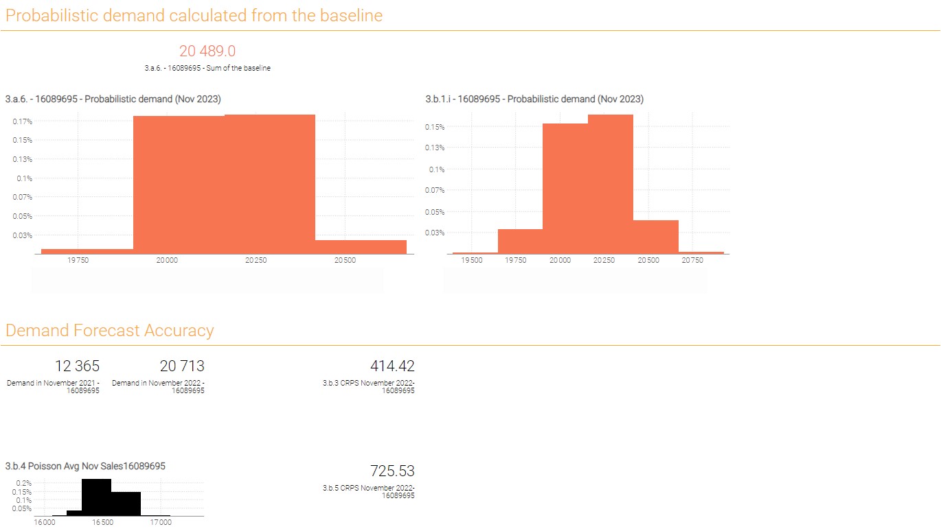
Note: Looking at the probabilistic demand histograms one might conclude there is an error as probability scale is so small that visually all bins don’t build up to 100% probability as they should. This conclusion however would be wrong. In the Envision environment hover your mouse over the bins and you will see that they consist out of many smaller bins with individual probabilities and the cumulative probability will be provided in the parenthesis. This unusual look of the distribution is a consequence of optimizing probabilistic forecast computations for both computational efficiency and accuracy. Usually these wide bin artifacts are the consequence of presence of lot multipliers and hint the boundaries of feasible decisions.
Conclusion
This exercise has provided a comprehensive understanding of the complexities involved in supply chain forecasting. It also demonstrates the importance of demand and leadtime forecasting in managing inventory levels, avoiding stock-outs, and ensuring customer satisfaction.
Key takeaways
Sales forecasting is not applying one single model/technique over and over.
Forecasting is not just about predicting future sales based on past data, rather it is foremost about understanding the core business factors that influence demand, such as seasonality, trends, products’ lifecycles, etc. It is also key to understand which data is available and what hypotheses can be made with it. For instance, the absence of a stock-out history can be the most significant contributor to forecasting inaccuracies.
As demand drivers are different from one company to another, it is crucial to use forecasting technologies that encompass modeling flexibility such as differentiable programming, the latter allowing one to craft models that can be easily adapted over time.
Don’t avoid uncertainty, embrace it!
A point-forecast approach is not adapted to the real issues one encounters in supply chain. Uncertainty is everywhere, be it delivery lead times, quantities sold, etc. As the core challenge is to handle these classes of problems (i.e., the tough cases), Lokad uses only probabilistic forecasts.
Focus on decisions (not forecast accuracy).
In the classic supply chain approach, measuring and improving forecasting accuracy is generally a critical objective. From Lokad’s perspective, this approach doesn’t solve real world issues because what really matters is the quality of your supply chain decisions.
For example, if demand over the next month is around 10 units, but in the meantime the supplier imposes an MOQ of 100 units, spending hours of effort to know whether the demand will be closer to 9 units or to 11 units is not relevant. That’s why Lokad recommends checking the quality of the decisions made (measured in financial terms, such as Dollars or Euros) rather than forecast accuracy.
That said, if measuring forecast accuracy really matters to a given situation, then choosing a metric that embraces the probabilistic approach should be considered.
Annex
Get the dataset from the Envision playground
/// ## 0.1 Reading data tables
read "/Catalog.tsv" as Items[Id] with
  /// The primary key, identifies each item.
  "Ref" as Id : text
  Name : text
  Category : text
  SubCategory : text
  Brand : text
  Supplier : text
  /// Unit price to buy 1 unit from the supplier.
  BuyPrice : number
  /// Unit price to sell 1 unit to to a client.
  SellPrice : number
  RLT : number

read "/Orders.tsv.gz"  as Sales expect [Id,Date] with
  /// Foreign key to `Items`.
  "Ref" as Id : text
  ///The date when the sales orders happened
  "OrderDate" as Date : date
  /// Where (Localisation) the sale took place
  Loc : text
  ///The quantity delivered to the customer
  DeliveryQty : number
  LokadNetAmount : number
read "/StockOut.tsv"  as Stockout expect[Id, Date] with
  /// Foreign key to `Items`.
  Id : text
  ///The date when the stock out happened
  Date : date
  IsStockOut : boolean
read "/ExtendedSLT.tsv" as ExtendedSLT expect [Id] with
  /// Foreign key to `Items`.
  "Ref" as Id : text
  Value : number
  SLTWeight:number


//// ## 0.2 Set of colors definition

colorDemand       = "blue"
colorSmoothDemand = "#7373EE"
colorBaseline     = "green"
mainColor = rgb(0.992, 0.678, 0.192)
bmainColor = rgb(0.973, 0.459, 0.318)
mgreen = rgb(0.416, 0.8, 0.392)
mred = rgb(0.839, 0.373, 0.373)
mblue = rgb(0.282, 0.471, 0.816)
myellow = rgb(0.835, 0.733, 0.404)
adark = rgb(0.89, 0.529, 0.0275)
alight = rgb(0.945, 0.855, 0.675)

/// ## 0.3 Introduction
show label "Demand Forecast" a1g1 {textAlign: center ; textBold: "true"}
show markdown "Generic Documentation" a2g2 with """
  Hi there, welcome to your fourth Envision exercise! Here, you will build a demand forecast.
  You'll start by a classic approach creating a point forecast. Then you will embrace the probabilistic approach
  and discover some advanced concepts of the Quantitative Supply Chain!
  """
/// ## 0.4 Supplier Lead times computation as it is a given random variable for the workshop

Items.SLT = mixture(dirac(ExtendedSLT.Value),ExtendedSLT.SLTWeight)

/// ## 0.5 Displaying raw Data tables
show table "Items" a3b3  with
  Items.Id
  Items.Brand as "Brand"
  Items.BuyPrice as "BuyPrice"
  Items.Category as "Category"
  Items.Name as "Name"
  Items.RLT as "RLT"
  Items.SellPrice as "SellPrice"
  Items.SubCategory as "SubCategory"
  Items.Supplier as "Supplier"
  Items.SLT


show table "Sales" c3d3  with
  Sales.Id as "Id"
  Sales.Date as "date"
  Sales.Loc as "Loc"
  Sales.DeliveryQty as "DeliveryQty"
  Sales.LokadNetAmount as "LokadNetAmount"

show table "Stockout" e3f3  with
  Stockout.Id as "Id"
  Stockout.date as "date"
  Stockout.IsStockOut as "IsStockOut"
  Stockout.Id as "Id"
  Stockout.date as "date"


///# ---------------- [Part I. Exploring the dataset & the business context ] -------------------

//Useful code and variables for the Part I

firstOrderDate = monday(min(Sales.Date)) + 7 // the first monday of full week of sale
lastOrderDate  = monday(max(Sales.Date)) - 7 // the last monday of full week of sale

///# ----------------- [Part II. Building a Deterministic Forecasting Model ] -----------------

//Useful Code to generate a single point model

///Question 2.a.1

keep where Date >= firstOrderDate
keep span Date = [firstOrderDate .. lastOrderDate + 2 * 365]
table Slices [slice] =
slice by Items.Id title: Items.Id

table ItemsWeek = cross(Items, Week)
ItemsWeek.Monday = monday(ItemsWeek.week)
ItemsWeek.TimeIndex = rankrev () by Items.Id scan -ItemsWeek.Monday

Items.SalesAmount365 = sum(Sales.LokadNetAmount) when(Sales.Date > lastOrderDate - 365)
Items.RankSalesAmount365 = rankrev () scan Items.SalesAmount365

keep where Items.SalesAmount365 > 0 //we only keep references with historical sales

/// Formula used to compute a smoothed sales
ItemsWeek.DemandQty = sum(Sales.DeliveryQty)
ItemsWeek.DemandQtyShiftM1 = ItemsWeek.DemandQty[-1] ///// [Week W-1]
ItemsWeek.DemandQtyShiftP1 = ItemsWeek.DemandQty[1] ///// [Week W+1]
ItemsWeek.DemandQtyShiftM2 = ItemsWeek.DemandQty[-2] ///// [Week W-2]
ItemsWeek.DemandQtyShiftP2 = ItemsWeek.DemandQty[2] ///// [Week W+2]
ItemsWeek.SmoothedDemand =
    if ItemsWeek.Monday == lastOrderDate then //last week of sales history
      0.1 * ItemsWeek.DemandQtyShiftM2 +
      0.2 * ItemsWeek.DemandQtyShiftM1 +
      0.7 * ItemsWeek.DemandQty
    else if ItemsWeek.Monday == lastOrderDate - 7 then //the week before the last week of sales history
      0.1 * ItemsWeek.DemandQtyShiftM2 +
      0.2 * ItemsWeek.DemandQtyShiftM1 +
      0.4 * ItemsWeek.DemandQty +
      0.3 * ItemsWeek.DemandQtyShiftP1
    else
      0.1 * ItemsWeek.DemandQtyShiftM2 +
      0.2 * ItemsWeek.DemandQtyShiftM1 +
      0.4 * ItemsWeek.DemandQty +
      0.2 * ItemsWeek.DemandQtyShiftP1 +
      0.1 * ItemsWeek.DemandQtyShiftP2

show linechart same("2.a.1. - Smoothed Demand Vs Demand - PN: \{Id}")by slice a5e8 slices:slice {tileColor: #(bmainColor)} with
  same(ItemsWeek.DemandQty) as "Demand"    {seriesPattern: dotted ; color: #(colorDemand)}
  same(ItemsWeek.SmoothedDemand) as "SmoothedDemand"  {color: #(colorSmoothDemand)}
  group by ItemsWeek.week

///Question 2.a.2

Items.FirstSale = min(Sales.Date) // considering an Item is launched at its first sale
Items.TotalWeekNb = week(lastOrderDate) - week(Items.FirstSale)
ItemsWeek.WeekNum = (ItemsWeek.week) - week(Items.FirstSale)
ItemsWeek.ItemLifeWeight = 0.3 + 1.2* (ItemsWeek.WeekNum / Items.TotalWeekNb)^(1/3)
topRef1 = same(Items.Id) when(Items.RankSalesAmount365 == 1)
show linechart "2.a.2 - Weight function by week" f5g8 { tileColor: #(bmainColor)}  with
  same(ItemsWeek.ItemLifeWeight) when(Items.RankSalesAmount365 == 1) as "Top Ref \{topRef1}" {color: #(adark)}
  group by ItemsWeek.Monday

///Question 2.b

Items.AverageSalePerWeek = sum(Sales.DeliveryQty) when(Date > lastOrderDate - 365) / 52
Items.Level =  max(0, log(Items.AverageSalePerWeek) )

///Question 2.c  ---------- First Deterministic Model ----------

/// --------------- Code lines for “CODE BLOCK #1: FIRST AUTODIFF MODEL”.  --------------- ///
///### ----------------------------- CODE BLOCK #1: FIRST AUTODIFF MODEL ----------------------------- ///

/// Define interval used for calculating the loss
ItemsWeek.IsCache = (ItemsWeek.Monday >= Items.FirstSale ) and ItemsWeek.Monday  < lastOrderDate
ItemsWeek.Cache = if ItemsWeek.IsCache then 1 else 0

/// Define interval for an Item
ItemsWeek.ItemIsLife = if (ItemsWeek.Monday >= Items.FirstSale )  then 1 else 0
ItemsWeek.CumSumLife = 0
where ItemsWeek.Monday >= Items.FirstSale
  ItemsWeek.CumSumLife = (sum(ItemsWeek.ItemIsLife) by ItemsWeek.Id scan ItemsWeek.week) - 1 where ItemsWeek.Monday >= Items.FirstSale

levelShiftMin = -1
levelShiftMax = 1

expect table Items max 300000
expect table ItemsWeek max 1000000

table YearWeek1[YearWeek1] max 52 = by ((Week.week  - week(firstOrderDate)) mod 52)

/// In this model we use the category for seasonnality groups
table Groups[Category1] = by Items.Category
table SeasonYW max 1m = cross(Groups, YearWeek1)

/// Number of iteration
maxEpochs = 400

where Date <= lastOrderDate
  autodiff Items epochs:maxEpochs learningRate:0.01 with
    params Items.Level in [0..20]
    params Items.Affinity1   in [0..] auto(0.5, 0.05)
    params SeasonYW.Profile1   in [0..1] auto(0.5, 0.1)
    params Items.LevelShift in [levelShiftMin..levelShiftMax]  auto(0, 0.05)

    a1 =  Items.Affinity1
    YearWeek1.SeasonalityModel = SeasonYW.Profile1 * a1
    Week.LinearTrend = ItemsWeek.Cache * ( 1 + ItemsWeek.CumSumLife * Items.LevelShift / 10)
    Week.Baseline = exp(Items.Level) * YearWeek1.SeasonalityModel * ItemsWeek.Cache * Week.LinearTrend
    Week.Coeff = ItemsWeek.Cache * ItemsWeek.ItemLifeWeight
    Week.DeltaSquare = (Week.Baseline - ItemsWeek.SmoothedDemand)^2

    /// Error Calculation
    Sum = sum(Week.Coeff * Week.DeltaSquare)/100

    return (Sum ;  Sum: Sum)

/// Retrieval of the results
table ItemsYW = cross(Items, YearWeek1)
ItemsYW.Category1 = Items.Category1
ItemsWeek.YearWeek1 = Week.YearWeek1

Items.SumAffinity = Items.Affinity1

ItemsYW.Profile1 = SeasonYW.Profile1

ItemsYW.SeasonalityModel = ItemsYW.Profile1  * Items.SumAffinity
// Trend reconstruction
ItemsWeek.LinearTrend =  max(0, 1 + (ItemsWeek.CumSumLife * Items.LevelShift /10))

ItemsWeek.CappingTrend = same(ItemsWeek.LinearTrend) when(ItemsWeek.week == week(52 * 7 + lastOrderDate )) by Id

ItemsWeek.TrendFinal = if ItemsWeek.Monday <= 52 * 7 + lastOrderDate  then
                             ItemsWeek.LinearTrend
                        else
                             ItemsWeek.CappingTrend

ItemsWeek.Baseline = exp(Items.Level) * ItemsYW.SeasonalityModel * ItemsWeek.TrendFinal

///### ----------------------------- End CODE BLOCK #1 ----------------------------- ///

// This following line allows you to select a reference and update reporting according to this reference

// show label same("\{Id} - Forecast") by slice a9g10  tileColor: #(mainColor)}
// show slicepicker "Select a Reference" h1i2 {tileColor: #(mainColor)} with
//   same(Items.Id ) as "Ref"

///Question 2.d

///### ----------------------------- CODE BLOCK #2 : SECOND AUTODIFF MODEL ----------------------------- ///

ItemsWeek.DemandQty = sum(Sales.DeliveryQty)
ItemsWeek.DemandQtyShiftM1 = ItemsWeek.DemandQty[-1]
ItemsWeek.DemandQtyShiftP1 = ItemsWeek.DemandQty[1]
ItemsWeek.DemandQtyShiftM2 = ItemsWeek.DemandQty[-2]
ItemsWeek.DemandQtyShiftP2 = ItemsWeek.DemandQty[2]

ItemsWeek.SmoothedDemand =
    if ItemsWeek.Monday == lastOrderDate then //last week of sales history
      0.1 * ItemsWeek.DemandQtyShiftM2 +
      0.2 * ItemsWeek.DemandQtyShiftM1 +
      0.7 * ItemsWeek.DemandQty
    else if ItemsWeek.Monday == lastOrderDate - 7 then //the week before the last week of sales history
      0.1 * ItemsWeek.DemandQtyShiftM2 +
      0.2 * ItemsWeek.DemandQtyShiftM1 +
      0.4 * ItemsWeek.DemandQty +
      0.3 * ItemsWeek.DemandQtyShiftP1
    else
      0.1 * ItemsWeek.DemandQtyShiftM2 +
      0.2 * ItemsWeek.DemandQtyShiftM1 +
      0.4 * ItemsWeek.DemandQty +
      0.2 * ItemsWeek.DemandQtyShiftP1 +
      0.1 * ItemsWeek.DemandQtyShiftP2

/// Define interval used for calculating the lost
ItemsWeek.IsCache = (ItemsWeek.Monday >= Items.FirstSale ) and ItemsWeek.Monday  < lastOrderDate
ItemsWeek.Cache = if ItemsWeek.IsCache then 1 else 0

/// Define interval for an Item
ItemsWeek.ItemIsLife = if (ItemsWeek.Monday >= Items.FirstSale )  then 1 else 0
ItemsWeek.CumSumLife = 0
where ItemsWeek.Monday >= firstOrderDate
  ItemsWeek.CumSumLife = (sum(ItemsWeek.ItemIsLife) by ItemsWeek.Id scan ItemsWeek.week) - 1 where ItemsWeek.Monday >= firstOrderDate

levelShiftMin = -1
levelShiftMax = 1

expect table Items max 300000
expect table ItemsWeek max 1000000

table YearWeek2[YearWeek2] max 52 = by ((Week.week  - week(firstOrderDate)) mod 52)
table GroupsSubCategory[SeasonDefinitionGroup] = by Items.Category
// / Correction

table SeasonYW2 max 1m = cross(GroupsSubCategory, YearWeek2)

// / Number of iteration
maxEpochs = 400

where Date <= lastOrderDate
  autodiff Items epochs:maxEpochs learningRate:0.01 with
    params Items.Level in [0..20]
    /// First Profil
    params Items.Affinity1   in [0..] auto(0.5, 0.05)
    params SeasonYW2.Profile1   in [0..1] auto(0.5, 0.1)
    params Items.LevelShift in [levelShiftMin..levelShiftMax]  auto(0, 0.05)


    a1 =  Items.Affinity1
    YearWeek2.SeasonalityModel = SeasonYW2.Profile1 * a1
    Week.LinearTrend = ItemsWeek.Cache * ( 1 + ItemsWeek.CumSumLife * Items.LevelShift / 10)
    Week.Baseline = exp(Items.Level) * YearWeek2.SeasonalityModel * ItemsWeek.Cache * Week.LinearTrend
    Week.Coeff = ItemsWeek.Cache * ItemsWeek.ItemLifeWeight
    Week.DeltaSquare = (Week.Baseline - ItemsWeek.SmoothedDemand)^2


    /// Error Calculation
    Sum = sum(Week.Coeff * Week.DeltaSquare)/100
    return (Sum ;  Sum: Sum)

// / Retrieval of the results
table ItemsYW2 = cross(Items, YearWeek2)
ItemsYW2.SeasonDefinitionGroup = Items.SeasonDefinitionGroup
ItemsWeek.YearWeek2 = Week.YearWeek2

ItemsYW2.Profile1 = SeasonYW2.Profile1

ItemsYW2.SeasonalityModel = (ItemsYW2.Profile1 * Items.Affinity1)

/// Trend reconstruction
ItemsWeek.LinearTrend =  max(0, 1 + (ItemsWeek.CumSumLife * Items.LevelShift /10))
ItemsWeek.CappingTrend = same(ItemsWeek.LinearTrend) when(ItemsWeek.week == week(52 * 7 + lastOrderDate )) by Id
ItemsWeek.TrendFinal = if ItemsWeek.Monday <= 52 * 7 + lastOrderDate  then
                         ItemsWeek.LinearTrend
                    else
                         ItemsWeek.CappingTrend

ItemsWeek.Baseline = exp(Items.Level) * ItemsYW2.SeasonalityModel * ItemsWeek.TrendFinal
///### ----------------------------- End CODE BLOCK #2 ----------------------------- //

///# ------------------------------ [Part III. Probabilistic approach and applications ] ---------------------------------

///Useful variables for Part III

TalonCotexSLTQ90 = 50
RLT = 30
Items.OLTConvertedInTimeIndex = round(Items.RLT/7) // we assume 4 steps of TimeIndex = approximately 1 full month of november

highSeasonStartDate = date(2023,10,30)
highSeasonEndDate   = date(2023,12,31)
mondayFirstOrder = monday(highSeasonStartDate - round(TalonCotexSLTQ90))
mondaySecondOrder = monday(highSeasonStartDate - round(TalonCotexSLTQ90) + RLT)
Week.Monday = monday(Week.week)

///Question 3.a.6

///### ----------------------------- N3: Probabilistic Demand ----------------------------- ///

focusRef = "16089695"
where Items.Id == focusRef
  Items.DispersionPerWeek = 1


  where ItemsWeek.Monday >= highSeasonStartDate
    ItemsWeek.TimeIndex = rankrev () by Items.Id scan -ItemsWeek.Monday
    Items.ProbabilisticDemandOverNov2023_1 = actionrwd.segment(
      TimeIndex: ItemsWeek.TimeIndex,
      BaseLine: ItemsWeek.Baseline,
      Dispersion: Items.DispersionPerWeek,
      Alpha: 0,
      Start: dirac(1),
      Duration: dirac(Items.OLTConvertedInTimeIndex),
      Samples : 1000)

  show scalar "3.a.6. - \{focusRef} - Probabilistic demand (Nov 2023)" a11d14  { tileColor: #(bmainColor)} with same(Items.ProbabilisticDemandOverNov2023_1)
// ///### ----------------------------- End N3 ----------------------------- ///

// show scalar "3.a.6. - \{focusRef} - Sum of the baseline" a10d10 {textAlign: center ;  tileColor: #(bmainColor)} with
  // sum(ItemsWeek.Baseline) when(Week.Monday >= highSeasonStartDate and Week.Monday < date(2023,11,27))

///Question 3.b.1

///### ----------------------------- N4: Probabilistic Demand ----------------------------- ///

where Items.Id == focusRef
  Items.DispersionPerWeek = dispersion(ranvar(ItemsWeek.Baseline)
                            when(highSeasonStartDate <= ItemsWeek.Monday and
                            ItemsWeek.Monday <= highSeasonStartDate + Items.OLTConvertedInTimeIndex))
  Items.DispersionPerWeek = max(1, Items.DispersionPerWeek)


  where ItemsWeek.Monday >= highSeasonStartDate
    ItemsWeek.TimeIndex = rankrev () by Items.Id scan -ItemsWeek.Monday
    Items.ProbabilisticDemandOverNov2023_2 = actionrwd.segment(
      TimeIndex: ItemsWeek.TimeIndex,
      BaseLine: ItemsWeek.Baseline,
      Dispersion: Items.DispersionPerWeek,
      Alpha: 0.2,
      Start: dirac(1),
      Duration: dirac(Items.OLTConvertedInTimeIndex),
      Samples : 2000)

  show scalar "3.b.1.i - \{focusRef} - Probabilistic demand (Nov 2023)" e11g14  {tileColor: #(bmainColor)} with same(Items.ProbabilisticDemandOverNov2023_2)

///### ----------------------------- End N4 ----------------------------- ///

///===============================================================================================///